FINANCIAL STATISTICS

Financial statistics include all numerical data that summarizes past behavior or forecasts future behavior of an individual financial security, a group of securities, or markets in a broad geographic region. It is useful to first categorize these statistics into one of three areas. Global or national statistics examine the behavior of business or economic conditions that influence the value of securities in general. Market or industrial statistics track the activity of a specific set of securities linked by a common trading market or industry classification. Company-specific statistics examine performance of individual firms.

GLOBAL/NATIONAL FINANCIAL
STATISTICS

ECONOMIC INDICATORS.

One broad class of global or national statistics is the series of economic indicators. These indicators assess where the economy is within the current business cycle and provide information useful to forecast the likelihood of improvement or deterioration, or to confirm the economy's current status. The National Bureau of Economic Research tracks several hundred measures of economic activity that are correlated with the status of the national economy. Economic indicators are typically split into three categories. Leading economic indicators correlate with patterns of future economic activity. For example, profit margins and the formation of new businesses tend to improve or deteriorate in advance of other symptoms of a change in the overall status of the economy. Coincident indicators assist in confirming of the economy's current status. Examples of these indicators are comprehensive levels of employment and industrial production. Finally, lagging indicators confirm that the economy has passed through a particular phase of the business cycle. Such indicators react after the change in economic condition has already been established. The average duration of unemployment is one example of a lagging indicator.

GROSS DOMESTIC PRODUCT.

There are many other examples of global economic statistics that have immediate relevance to financial analysis. One commonly followed statistic is the forecasted growth rate in gross domestic product (GDP). As an aggregate measure of overall output of a national economy, GDP growth is a highly anticipated figure. Many of the subcategories of GDP, such as government spending and exports, are closely followed as well.

EXCHANGE RATE STATISTICS.

A more pervasive and continuous source of financial information is found in exchange rate statistics. An exchange rate is the price of one country's currency in terms of another's. For example, if the U.S. dollar can be exchanged for 5 French francs, then residents in either country can quickly assess the value of real or financial assets in the other country. Since this data is so important to international trade and capital flows, exchange rate statistics are widely reported in many periodicals and newspapers on a daily basis.

INTEREST RATES.

Another set of statistics that are broadly followed in financial markets throughout the world are those associated with interest rates. Interest rates represent the price of money in a particular currency. This price includes a premium for expected inflation and another premium for risk of default. One common method of reporting interest rates is the yield curve. The yield curve represents the relationship between the maturity of a debt instrument, typically bonds, and the rate of return implied by its current price. A yield curve represents a relevant comparison of yields between different securities with different maturities only if the securities have similar default risk. As a result, the most common yield curve statistics relate to government bonds within a particular country. These statistics are frequently reported in tabular form with yields on various securities sorted by maturity. The same information is also commonly depicted in a graph. For example, early 1999 yields for U.S. Treasury bonds with maturities of 1, 5, 10, 20, and 30 years are 5.08 percent, 5.33 percent, 5.61 percent, 5.89 percent, and 5.62 percent, respectively. With the exception of the 30-year bond, this pattern is indicative of an upward sloping yield curve. This is the most common pattern, but inverted and humped yield curves have also been observed during the past two decades. Similar statistics can be graphed for corporate bonds with similar default risk ratings.

MARKET/INDUSTRIAL FINANCIAL
STATISTICS

The second broad category of financial statistics assesses the behavior of security markets. Most countries with well-developed financial markets have a variety of indexes that track overall market activity or activity of a specific market segment. Examples of these indexes in the United States are the Dow Jones Industrial Average, the Standard & Poor's 500, and the New York Stock Exchange Composite. Other examples include the Financial Times 100 in the United Kingdom, the Nikkei 225 in Japan, and the CAC 40 in France. Each of these widely followed indexes tracks general market conditions. Market indexes can be distinguished by their method of construction or the sample of securities they comprise.

There are three basic techniques for construction of market indexes. A price-weighted index basically reports the average price per share for a sample of securities. A value-weighed index monitors changes in the aggregate market value of all shares outstanding for a sample of securities. An equally weighted index determines the change in value for each security separately and then reports the average change for all securities. Value-weighted and equally weighted indexes are expressed as a proportion of some base value determined at a particular point in time. The proportion is often multiplied by a number such as 100 before it is reported.

The Dow Jones Industrial Average (DJIA) is an example of a price-weighted index. This means that the index tracks and reports the average price per share of a sample of securities. The DJIA has been in existence since 1885 when it was first constructed by Charles Dow. He selected 20 "blue chip," or well-established, companies and tracked the average price per share. In the late 1920s, the number of stocks was increased to 30. During the more than 100 years of its existence, many DJIA stocks have split (i.e., issued two new shares to replace one old share) when management felt that their share price had become exorbitant. In addition, some firms have gone bankrupt or merged with other firms and thus trading in these securities has been eliminated. A price-weighted average accounts for such changes by altering the divisor to render the event neutral. Through this technique, the divisor of the DJIA, which was 30 in the late 1920s, had fallen to 0.23006576 by 1999.

As statistics of aggregate market behavior, price-weighted averages suffer from several biases. For example, a high price-per-share stock has greater influence over the index than a lower price-per-share stock even though there may be many more shares of the lower priced stock outstanding. In addition, stocks split to reduce price per share and make them more affordable to investors. A split does not alter the collective value of the stock (i.e., 100 shares at $10 are worth the same as 200 shares at $5), but it does reduce the impact of that stock on the overall index. This is relevant since it is the stocks with the highest growth that have the greatest propensity to split and implies that price-weighted averages are downwardly biased indicators of market performance. The DJIA in particular is frequently criticized for its small sample of purely industrial firms. This suggests that it may be a poor proxy for overall market behavior. Statistical analysis indicates, however, that it is highly correlated with other, broader measures of market activity.

The Standard & Poor's 500 (S&P 500) is a value-weighted index that comprises a sample of 400 industrial, 20 transportation, 40 utility, and 40 financial firms. It is constructed by multiplying the current share price by the number of shares outstanding for each of its 500 firms. The sum of these products is divided by a similar sum constructed using stock prices from the period from 1941 to 1943. This ratio represents the cumulative growth of this portfolio of 500 stocks from that base period to the current period. Unlike the price-weighted average, stock splits are neutral events since the aggregate value of all shares of a firm is not changed by the split. Bankruptcies, mergers, and other events that stop public trading of a firm's stock will require adjustment of the index. While the S&P 500 comprises a much larger sample of securities, larger firms have a greater influence on its behavior. To see this more specifically, imagine ranking all 500 firms by value. Clearly, the largest firm will represent a much larger portion of the aggregate value of the entire sample of 500 firms than will the smallest.

The development of an equally weighted index is an attempt to eliminate the bias just described in the value-weighted index. The idea behind an equally weighted index is to generate a ratio, or growth factor, for an individual firm by measuring its stock price today and dividing by its stock price during some base period. This process is repeated for a sample of stocks and then an average growth factor is reported. One such index that represents approximately 1,700 U.S. stocks is the Value Line Index. Equally weighted measures are considered a better measure of the behavior of the typical security during any period of time.

While this discussion has focused on stock indexes for the overall market, there are many other indexes that examine other classes of securities or specific industries or segments of the market. For example, the New York Stock Exchange also tracks a value-weighted average of its listed firms in the categories of industrials, utilities, transportation, and finance. Many publications use an even finer breakdown of industrial classifications. There are also a broad variety of indexes that examine various categories of bonds and mutual funds.

FIRM-SPECIFIC FINANCIAL STATISTICS

A final category of financial statistics are those that are firm specific. These statistics include bond ratings, price/earnings ratios, and other indicators of risk and return.

HISTORICAL STATISTICS.

It is useful to begin by considering statistics constructed from historical measures. For example, an analysis of periodic prices and cash payments from a historical period provides the data needed to construct statistics of risk and return. Historical returns can be reported as an arithmetic average (computing rate of return for a series of sequential periods and averaging) or a geometric average (computing the annualized compound interest rate that the investor would have received). Additionally, this data will allow for construction of risk statistics such as variance and standard deviation.

To illustrate the computation of these historical statistics, consider the following example that uses data for Coca-Cola. Table I contains the closing price for a share of Coca-Cola stock at the end of February for five consecutive years. It also contains the dividend per share that Coca-Cola paid during each year and the one-year holding period return—or the rate of return an investor would have achieved during that particular period.

The holding period return (HPR) for each one-year period is computed using the following formula:

In other words, the overall return from stock appreciation and dividend income from 1995 to 1996 was 48.4 percent. Similar interpretations can be derived from the calculation for subsequent years. We can average, or annualize these returns by adding the one-year HPR and then dividing by the number of returns—four in this example.

The other interesting observation that can quickly be drawn from the table of holding period returns is their significant volatility from year to year. This can be formally measured as variance or standard deviation, both important measures of risk. Variance of these returns can be computed by calculating the deviation of each individual annual holding period return from the mean return computed above, squaring this difference, adding the squared differences together and finally dividing by the number of years in the sample. The Coca-Cola data allows the following computation of variance:

The variance is an aggregate measure of dispersion away from the mean return. It is commonly restated as a standard deviation by computing its square root. In this example, the standard deviation of Coca-Cola's returns is 0.244 or 24.4 percent. Equipped with a mean to measure the security's return and a standard deviation to assess its risk, meaningful comparisons can now be made with other securities that have been subjected to similar analysis.

While the statistical measures constructed in the preceding example are valid, it is important to consider their purpose. If an investor was interested in performance over some prior time interval to answer questions such as "How well did my investment perform?" or "How much risk was I exposed to?," then these statistics are clear indicators. On the other hand, if an investor wants to know "How will this security perform?" or "How risky is this stock?," then the statistics must be interpreted quite differently. In the second case, the historical statistics are valuable only

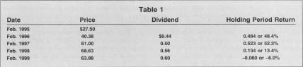
Date	Price	Dividend	Holding Period Return
Feb. 1995	S27.50
Feb. 1996	40.38	$0.44	0.484 or 48.4%
Feb. 1997	61.00	0.50	0.523 or 52.3%
Feb.1998	68.63	0.56	0.134 or 13.4%
Feb. 1999	63.88	0.60	-0.060 or -6.0%

if it is reasonable to expect future performance to correlate to past performance. It is usually reasonable to use historical risk as a proxy for expected risk. This is because risk is a function of exposure to broader economic forces and firm-specific characteristics such as financial structure and operating cost structure. These influences are not likely to change, or changes are reasonably predictable. Nevertheless, it is typically more difficult to use historical return as a proxy for expected future return.

The measure of risk can be refined by dividing total risk, as measured by standard deviation, into two parts. The first part is the variation in a stock's return that results from general market movements and is referred to as systematic risk. The second component is the variation that results from factors unique to the individual firm and is referred to as unsystematic risk. There is considerable interest in the systematic risk component of a stock's overall risk because the unsystematic risk can be minimized by holding a variety of securities together in a portfolio. Systematic risk is measured by the statistic beta (j). Beta represents the volatility of an individual security relative to the average market volatility. Therefore, the average security beta is 1. Beta can be derived statistically by computing the ratio of the covariance of the individual security's returns with those of the market by the variance of the market's returns. It can also be derived by the regression procedure where the equation of the line that best fits a scatter of points—each representing return for the security and the market at a particular point in time—is determined statistically. The slope of this line represents the security's beta. Beta is a useful statistic in portfolio management because it allows managers to actively position their portfolios in an above-average, average, or below-average risk position by choosing securities with an average beta of above 1, exactly 1, or below 1, respectively.

FINANCIAL RATIOS.

A final category of firm-specific statistics refers to the financial statements that the firm has generated in the past and allows forecasts of future financial performance. Financial ratios comprise another family of relevant statistics that are frequently used to assess the financial health and development of individual firms. While some of the more prominent financial ratios relate to profitability (e.g., net profit margin, return on equity), others can be used to assess other characteristics of a firm that ultimately pinpoint potential reasons for the resulting profitability. These other measures can be categorized into several areas. Liquidity ratios assess the firm's ability to meet its short-term financial obligations with its most liquid assets. Activity ratios measure how effectively the firm is able to use various categories of assets to generate sales revenues. Leverage ratios examine how the firm's assets are financed and how the firm's financing structure is likely to influence profits. Finally, there are many ratios that attempt to relate market values of the firm's assets to their financial statement counterparts. Collectively, these ratios can be monitored over time to detect trends in firm performance or they can be examined in relation to industry average ratios. In either case, the statistics can be very useful for probing, explaining, and forecasting a firm's financial performance.