EXPECTED VALUE

Expected value is a statistical concept that is applied to many business situations. Often, the term may be loosely used. Nevertheless, whenever someone mentions expected profit or expected loss from a business venture—that is, the expected value of the likely magnitude of profit or loss from the business under consideration—the term has a rigorous mathematical foundation.

DEFINING EXPECTED VALUE

The expected value concept uses two main mathematical concepts—random variables and probabilities. To understand a random variable, let us assume that an experiment results in a certain number of outcomes and each of the outcomes is assigned a numerical value. A random variable then is a numerical description of the outcome of an experiment. Suppose a coin is tossed. In this case, there are two possible outcomes: heads or tails. One can assign a numerical value of 1 with the outcome heads and a value of 0 with outcome tails. Thus, if we consider the number of possible outcomes on a single toss as a random variable (often given a generic mathematical name x), it takes two values: x = 0, 1. In a more complicated case, a random variable can take a large number of values—sometimes even an infinite number of values.

The notion of probability is quite widely used and refers to the chance of an event occurring. The probability of an event (denoted as p) lies between 0 and 1. That is, 0 is less than or equal to p and p is less than or equal to 1. In the above example of coin tossing, the probability of heads turning up on a toss is 0.5 and the probability of tails turning up is also 0.5.

One may be able to assign a probability value to every value a random variable takes. In the preceding example, one can say that the probability that x = 1 is 0.5. Mathematically, it can be said that p(x) = 0.5 when x = 1 (when heads turns up). Similarly, one can say that p(x) = 0.5 when x = 0 (when tails turns up).

A mathematical expression for the expected value of a random variable (x) can now be given as:

In this expression, the notation E is the Greek letter capital sigma. Mathematicians use the X notation to indicate sum of a number of items. E(x) is used as a notation for the expected value of the random variable x, and p(x) is the probability that the random variable x takes a particular value. The above expression thus holds that in order to compute the expected value of a discrete random variable, one must multiply each value of the random variable by its corresponding probability and then add all the resulting products. For the tossed coin example, the expected value (that is, the expected number of heads on a toss) can be calculated as follows using the above expression: 1 * 0.5 + 0 * 0.5 = 0.5. Here, the random variable takes two values: 1 (a head) and 0 (a tail) with probabilities 0.5 each. The expected value calculation implies that the expected number of heads on a single toss is 0.5. This means that if one tosses a coin 100 times, one would expect to see 50 heads on the basis of the expected value concept.

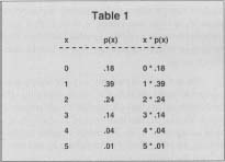
Since the coin example is a rather simple one, a more realistic example follows. Suppose that we have data on the number of children that American families have (call it the random variable x). The minimum number of children a family had was 0 and the maximum number of children a family had was 5. Thus, the random variable x takes six values: x equals 0,1,2, 3, 4 and 5. Based on the number of families with different numbers of children, one has data on the probability of a family having a certain number of children. These data are provided in the first two columns of Table 1.

X	P(x)	X *P(x)
0	.18	0 *.18
1	.39	1 *.39
2	.24	2 *.24
3	.14	3 *.14
4	.04	4 *.04
5	.01	5 *.01

The first two columns of Table 1 show that the probability of a family having 0 number of children is equal to 0.18 or 18 percent. Similarly, the probability of a family having 1 child is equal to 0.39 or 39 percent; the probability of a family having 2 children is equal to 0.24 or 24 percent; the probability of a family having 3 children is equal to 0.14 or 14 percent; the probability of a family having 4 children is equal to 0.04 or 4 percent; and the probability of a family having 5 children is equal to 0.01 or 1 percent. The last column of the table multiplies the different values of x by its corresponding probability, according to the previously given mathematical expression, to compute the expected value of the number of children in those households to whom the above data apply. When all the six products are added, the expected value of the number of children (that is, the expected value of the random variable x) turns out to be 1.5. One can interpret the expected value of 1.5 as the mean number of children for the households considered. In more concrete terms, we can say that if a family was picked at random from among the families considered, it would be expected to have 1.5 children.

The application of the expected value concept to business can be illustrated using the following example. Suppose a business firm has the option of building a plant of large, medium, or small size. Profits from each plant size depend on whether demand is low or high. Assume that the firm knows the probabilities of low and high demands. Based on these probabilities and corresponding profit/loss figures, the firm can calculate the expected profit for each plant size. The firm should build the plant that generates the largest expected profits.