FORECASTING

Forecasting involves the generation of a number, set of numbers, or scenario that corresponds to a future occurrence. It is absolutely essential to short-range and long-range planning. By definition, a forecast is based on past data, as opposed to a prediction, which is more subjective and based on instinct, gut feel, or guess. For example, the evening news gives the weather "forecast" not the weather "prediction." Regardless, the terms forecast and prediction are often used inter-changeably. For example, definitions of regression—a technique sometimes used in forecasting—generally state that its purpose is to explain or "predict."
Forecasting is based on a number of assumptions:
- The past will repeat itself. In other words, what has happened in the past will happen again in the future.
- As the forecast horizon shortens, forecast accuracy increases. For instance, a forecast for tomorrow will be more accurate than a forecast for next month; a forecast for next month will be more accurate than a forecast for next year; and a forecast for next year will be more accurate than a forecast for ten years in the future.
- Forecasting in the aggregate is more accurate than forecasting individual items. This means that a company will be able to forecast total demand over its entire spectrum of products more accurately than it will be able to forecast individual stock-keeping units (SKUs). For example, General Motors can more accurately forecast the total number of cars needed for next year than the total number of white Chevrolet Impalas with a certain option package.
- Forecasts are seldom accurate. Furthermore, forecasts are almost never totally accurate. While some are very close, few are "right on the money." Therefore, it is wise to offer a forecast "range." If one were to forecast a demand of 100,000 units for the next month, it is extremely unlikely that demand would equal 100,000 exactly. However, a forecast of 90,000 to 110,000 would provide a much larger target for planning.
William J. Stevenson lists a number of characteristics that are common to a good forecast:
- Accurate—some degree of accuracy should be determined and stated so that comparison can be made to alternative forecasts.
- Reliable—the forecast method should consistently provide a good forecast if the user is to establish some degree of confidence.
- Timely—a certain amount of time is needed to respond to the forecast so the forecasting horizon must allow for the time necessary to make changes.
- Easy to use and understand—users of the forecast must be confident and comfortable working with it.
- Cost-effective—the cost of making the forecast should not outweigh the benefits obtained from the forecast.
Forecasting techniques range from the simple to the extremely complex. These techniques are usually classified as being qualitative or quantitative.
QUALITATIVE TECHNIQUES
Qualitative forecasting techniques are generally more subjective than their quantitative counterparts. Qualitative techniques are more useful in the earlier stages of the product life cycle, when less past data exists for use in quantitative methods. Qualitative methods include the Delphi technique, Nominal Group Technique (NGT), sales force opinions, executive opinions, and market research.
THE DELPHI TECHNIQUE.
The Delphi technique uses a panel of experts to produce a forecast. Each expert is asked to provide a forecast specific to the need at hand. After the initial forecasts are made, each expert reads what every other expert wrote and is, of course, influenced by their views. A subsequent forecast is then made by each expert. Each expert then reads again what every other expert wrote and is again influenced by the perceptions of the others. This process repeats itself until each expert nears agreement on the needed scenario or numbers.
NOMINAL GROUP TECHNIQUE.
Nominal Group Technique is similar to the Delphi technique in that it utilizes a group of participants, usually experts. After the participants respond to forecast-related questions, they rank their responses in order of perceived relative importance. Then the rankings are collected and aggregated. Eventually, the group should reach a consensus regarding the priorities of the ranked issues.
SALES FORCE OPINIONS.
The sales staff is often a good source of information regarding future demand. The sales manager may ask for input from each sales-person and aggregate their responses into a sales force composite forecast. Caution should be exercised when using this technique as the members of the sales force may not be able to distinguish between what customers say and what they actually do. Also, if the forecasts will be used to establish sales quotas, the sales force may be tempted to provide lower estimates.
EXECUTIVE OPINIONS.
Sometimes upper-levels managers meet and develop forecasts based on their knowledge of their areas of responsibility. This is sometimes referred to as a jury of executive opinion.
MARKET RESEARCH.
In market research, consumer surveys are used to establish potential demand. Such marketing research usually involves constructing a questionnaire that solicits personal, demographic, economic, and marketing information. On occasion, market researchers collect such information in person at retail outlets and malls, where the consumer can experience—taste, feel, smell, and see—a particular product. The researcher must be careful that the sample of people surveyed is representative of the desired consumer target.
QUANTITATIVE TECHNIQUES
Quantitative forecasting techniques are generally more objective than their qualitative counterparts. Quantitative forecasts can be time-series forecasts (i.e., a projection of the past into the future) or forecasts based on associative models (i.e., based on one or more explanatory variables). Time-series data may have underlying behaviors that need to be identified by the forecaster. In addition, the forecast may need to identify the causes of the behavior. Some of these behaviors may be patterns or simply random variations. Among the patterns are:
- Trends, which are long-term movements (up or down) in the data.
- Seasonality, which produces short-term variations that are usually related to the time of year, month, or even a particular day, as witnessed by retail sales at Christmas or the spikes in banking activity on the first of the month and on Fridays.
- Cycles, which are wavelike variations lasting more than a year that are usually tied to economic or political conditions.
- Irregular variations that do not reflect typical behavior, such as a period of extreme weather or a union strike.
- Random variations, which encompass all non-typical behaviors not accounted for by the other classifications.
Among the time-series models, the simplest is the naïve forecast. A naïve forecast simply uses the actual demand for the past period as the forecasted demand for the next period. This, of course, makes the assumption that the past will repeat. It also assumes that any trends, seasonality, or cycles are either reflected in the previous period's demand or do not exist. An example of naïve forecasting is presented in Table 1.
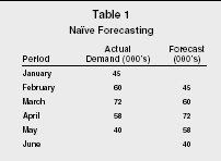
Naïve Forecasting
| Period | Actual Demand (000's) | Forecast (000's) |
| January | 45 | |
| February | 60 | 45 |
| March | 72 | 60 |
| April | 58 | 72 |
| May | 40 | 58 |
| June | 40 |
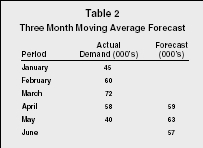
Another simple technique is the use of averaging. To make a forecast using averaging, one simply takes the average of some number of periods of past data by summing each period and dividing the result by the number of periods. This technique has been found to be very effective for short-range forecasting.
Variations of averaging include the moving average, the weighted average,
and the weighted moving average. A moving average takes a predetermined
number of periods, sums their actual demand, and divides by the number of
periods to reach a forecast. For each subsequent period, the oldest period
of data drops off and the latest period is added. Assuming a three-month
moving average and using the data from Table 1, one would simply add 45
(January), 60 (February), and 72 (March) and divide by three to arrive at
a forecast for April:
45 + 60 + 72 = 177 ÷ 3 = 59
To arrive at a forecast for May, one would drop January's demand from the equation and add the demand from April. Table 2 presents an example of a three-month moving average forecast.
Three Month Moving Average Forecast
| Period | Actual Demand (000's) | Forecast (000's) |
| January | 45 | |
| February | 60 | |
| March | 72 | |
| April | 58 | 59 |
| May | 40 | 63 |
| June | 57 |
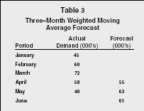
A weighted average applies a predetermined weight to each month of past
data, sums the past data from each period, and divides by the total of the
weights. If the forecaster adjusts the weights so that their sum is equal
to 1, then the weights are multiplied by the actual demand of each
applicable period. The results are then summed to achieve a weighted
forecast. Generally, the more recent the data the higher the weight, and
the older the data the smaller the weight. Using the demand example, a
weighted average using weights of .4, .3, .2, and .1 would yield the
forecast for June as:
60(.1) + 72(.2) + 58(.3) + 40(.4) = 53.8
Forecasters may also use a combination of the weighted average and moving average forecasts. A weighted moving average forecast assigns weights to a predetermined number of periods of actual data and computes the forecast the same way as described above. As with all moving forecasts, as each new period is added, the data from the oldest period is discarded. Table 3 shows a three-month weighted moving average forecast utilizing the weights .5, .3, and .2.
Three–Month Weighted Moving Average Forecast
| Period | Actual Demand (000's) | Forecast (000's) |
| January | 45 | |
| February | 60 | |
| March | 72 | |
| April | 58 | 55 |
| May | 40 | 63 |
| June | 61 |
A more complex form of weighted moving average is exponential smoothing,
so named because the weight falls off exponentially as the data ages.
Exponential smoothing takes the previous period's forecast and
adjusts it by a predetermined smoothing constant, ά (called alpha;
the value for alpha is less than one) multiplied by the difference in the
previous forecast and the demand that actually occurred during the
previously forecasted period (called forecast error). Exponential
smoothing is expressed formulaically as such:
New forecast = previous forecast + alpha (actual demand − previous
forecast)
F = F + ά(A − F)
Exponential smoothing requires the forecaster to begin the forecast in a
past period and work forward to the period for which a current forecast is
needed. A substantial amount of past data and a beginning or initial
forecast are also necessary. The initial forecast can be an actual
forecast from a previous period, the actual demand from a previous period,
or it can be estimated by averaging all or part of the past data. Some
heuristics exist for computing an initial forecast. For example, the
heuristic N = (2 ÷ ά) − 1 and an alpha of .5 would
yield an N of 3, indicating the user would average the first three periods
of data to get an initial forecast. However, the accuracy of the initial
forecast is not critical if one is using large amounts of data, since
exponential smoothing is "self-correcting." Given enough
periods of past data, exponential smoothing will eventually make enough
corrections to compensate for a reasonably inaccurate initial forecast.
Using the data used in other examples, an initial forecast of 50, and an
alpha of .7, a forecast for February is computed as such:
New forecast (February) = 50 + .7(45 − 50) = 41.5
Next, the forecast for March:
New forecast (March) = 41.5 + .7(60 − 41.5) = 54.45
This process continues until the forecaster reaches the desired period.
In Table 4 this would be for the month of June, since the actual demand
for June is not known.
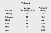
| Period | Actual Demand (000's) | Forecast (000's) |
| January | 45 | 50 |
| February | 60 | 41.5 |
| March | 72 | 54.45 |
| April | 58 | 66.74 |
| May | 40 | 60.62 |
| June | 46.19 |
An extension of exponential smoothing can be used when time-series data exhibits a linear trend. This method is known by several names: double smoothing; trend-adjusted exponential smoothing; forecast including trend (FIT); and Holt's Model. Without adjustment, simple exponential smoothing results will lag the trend, that is, the forecast will always be low if the trend is increasing, or high if the trend is decreasing. With this model there are two smoothing constants, ά and β with β representing the trend component.
An extension of Holt's Model, called Holt-Winter's Method, takes into account both trend and seasonality. There are two versions, multiplicative and additive, with the multiplicative being the most widely used. In the additive model, seasonality is expressed as a quantity to be added to or subtracted from the series average. The multiplicative model expresses seasonality as a percentage—known as seasonal relatives or seasonal indexes—of the average (or trend). These are then multiplied times values in order to incorporate seasonality. A relative of 0.8 would indicate demand that is 80 percent of the average, while 1.10 would indicate demand that is 10 percent above the average. Detailed information regarding this method can be found in most operations management textbooks or one of a number of books on forecasting.
Associative or causal techniques involve the identification of variables that can be used to predict another variable of interest. For example, interest rates may be used to forecast the demand for home refinancing. Typically, this involves the use of linear regression, where the objective is to develop an equation that summarizes the effects of the predictor (independent) variables upon the forecasted (dependent) variable. If the predictor variable were plotted, the object would be to obtain an equation of a straight line that minimizes the sum of the squared deviations from the line (with deviation being the distance from each point to the line). The equation would appear as: y = a + bx, where y is the predicted (dependent) variable, x is the predictor (independent) variable, b is the slope of the line, and a is equal to the height of the line at the y-intercept. Once the equation is determined, the user can insert current values for the predictor (independent) variable to arrive at a forecast (dependent variable).
If there is more than one predictor variable or if the relationship between predictor and forecast is not linear, simple linear regression will be inadequate. For situations with multiple predictors, multiple regression should be employed, while non-linear relationships call for the use of curvilinear regression.
ECONOMETRIC FORECASTING
Econometric methods, such as autoregressive integrated moving-average model (ARIMA), use complex mathematical equations to show past relationships between demand and variables that influence the demand. An equation is derived and then tested and fine-tuned to ensure that it is as reliable a representation of the past relationship as possible. Once this is done, projected values of the influencing variables (income, prices, etc.) are inserted into the equation to make a forecast.
EVALUATING FORECASTS
Forecast accuracy can be determined by computing the bias, mean absolute
deviation (MAD), mean square error (MSE), or mean absolute percent error
(MAPE) for the forecast using different values for alpha. Bias is the sum
of the forecast errors [∑(FE)]. For the exponential smoothing
example above, the computed bias would be:
(60 − 41.5) + (72 − 54.45) + (58 − 66.74) + (40
− 60.62) = 6.69
If one assumes that a low bias indicates an overall low forecast error, one could compute the bias for a number of potential values of alpha and assume that the one with the lowest bias would be the most accurate. However, caution must be observed in that wildly inaccurate forecasts may yield a low bias if they tend to be both over forecast and under forecast (negative and positive). For example, over three periods a firm may use a particular value of alpha to over forecast by 75,000 units (−75,000), under forecast by 100,000 units (+100,000), and then over forecast by 25,000 units (−25,000), yielding a bias of zero (−75,000 + 100,000 − 25,000 = 0). By comparison, another alpha yielding over forecasts of 2,000 units, 1,000 units, and 3,000 units would result in a bias of 5,000 units. If normal demand was 100,000 units per period, the first alpha would yield forecasts that were off by as much as 100 percent while the second alpha would be off by a maximum of only 3 percent, even though the bias in the first forecast was zero.
A safer measure of forecast accuracy is the mean absolute deviation (MAD).
To compute the MAD, the forecaster sums the absolute value of the forecast
errors and then divides by the number of forecasts (∑ |FE| ÷
N). By taking the absolute value of the forecast errors, the offsetting of
positive and negative values are avoided. This means that both an over
forecast of 50 and an under forecast of 50 are off by 50. Using the data
from the exponential smoothing example, MAD can be computed as follows:
(| 60 − 41.5 | + | 72 − 54.45 | + | 58 − 66.74 | + |
40 − 60.62 |) ÷ 4 = 16.35
Therefore, the forecaster is off an average of 16.35 units per forecast.
When compared to the result of other alphas, the forecaster will know that
the alpha with the lowest MAD is yielding the most accurate forecast.
Mean square error (MSE) can also be utilized in the same fashion. MSE is
the sum of the forecast errors squared divided by N-1 [(∑(FE))
÷ (N-1)]. Squaring the forecast errors eliminates the possibility
of offsetting negative numbers, since none of the results can be negative.
Utilizing the same data as above, the MSE would be:
[(18.5) + (17.55) + (−8.74) + (−20.62)] ÷ 3 = 383.94
As with MAD, the forecaster may compare the MSE of forecasts derived using
various values of alpha and assume the alpha with the lowest MSE is
yielding the most accurate forecast.
The mean absolute percent error (MAPE) is the average absolute percent
error. To arrive at the MAPE one must take the sum of the ratios between
forecast error and actual demand times 100 (to get the percentage) and
divide by N [(∑ | Actual demand − forecast |÷ Actual
demand) × 100 ÷ N]. Using the data from the exponential
smoothing example, MAPE can be computed as follows:
[(18.5/60 + 17.55/72 + 8.74/58 + 20.62/48) × 100] ÷ 4 = 28.33%
As with MAD and MSE, the lower the relative error the more accurate the
forecast.
It should be noted that in some cases the ability of the forecast to change quickly to respond to changes in data patterns is considered to be more important than accuracy. Therefore, one's choice of forecasting method should reflect the relative balance of importance between accuracy and responsiveness, as determined by the forecaster.
MAKING A FORECAST
William J. Stevenson lists the following as the basic steps in the forecasting process:
- Determine the forecast's purpose. Factors such as how and when the forecast will be used, the degree of accuracy needed, and the level of detail desired determine the cost (time, money, employees) that can be dedicated to the forecast and the type of forecasting method to be utilized.
- Establish a time horizon. This occurs after one has determined the purpose of the forecast. Longer-term forecasts require longer time horizons and vice versa. Accuracy is again a consideration.
- Select a forecasting technique. The technique selected depends upon the purpose of the forecast, the time horizon desired, and the allowed cost.
- Gather and analyze data. The amount and type of data needed is governed by the forecast's purpose, the forecasting technique selected, and any cost considerations.
- Make the forecast.
- Monitor the forecast. Evaluate the performance of the forecast and modify, if necessary.
SEE ALSO: Futuring ; Manufacturing Resources Planning ; Planning ; Sales Management
R. Anthony Inman
FURTHER READING:
Finch, Byron J. Operations Now: Profitability, Processes, Performance. 2 ed. Boston: McGraw-Hill Irwin, 2006.
Green, William H. Econometric Analysis. 5 ed. Upper Saddle River, NJ: Prentice Hall, 2003.
Joppe, Dr. Marion. "The Nominal Group Technique." The Research Process. Available from < http://www.ryerson.ca/~mjoppe/ResearchProcess/841TheNominalGroupTechnique.htm >.
Stevenson, William J. Operations Management. 8 ed. Boston: McGraw-Hill Irwin, 2005.
also just wanted to say thanks, ur site was very clear and helpful in understanding forecasting.
thanks again
mike