MANAGEMENT SCIENCE

Management science generally refers to mathematical or quantitative methods for business decision making. The term "operations research" may be used interchangeably with management science.
HISTORY
Frederick Winslow Taylor is credited with the initial development of scientific management techniques in the early 1900s. In addition, several management science techniques were further developed during World War II. Some even consider the World War II period as the beginning of management science.
World War II posed many military, strategic, logistic, and tactical problems. Operations research teams of engineers, mathematicians, and statisticians were developed to use the scientific method to find solutions for many of these problems.
Nonmilitary management science applications developed rapidly after World War II. Based on quantitative methods developed during World War II, several new applications emerged. The development of the simplex method by George Dantzig in 1947 made application of linear programming practical. C. West Churchman, Russell Ackoff, and Leonard Arnoff made management science even more accessible by publishing the first operations research textbook in 1957.
Computer technology continues to play an integral role in management science. Practitioners and researchers are able to use ever-increasing computing power in conjunction with management science methods to solve larger and more complex problems. In addition, management scientists are constantly developing new algorithms and improving existing algorithms; these efforts also enable management scientists to solve larger and more complex problems.
BREADTH OF MANAGEMENT SCIENCE
TECHNIQUES
The scope of management science techniques is broad. These techniques include:
- mathematical programming
- linear programming
- simplex method
- dynamic programming
- goal programming
- integer programming
- nonlinear programming
- stochastic programming
- Markov processes
- queuing theory/waiting-line theory
- transportation method
- simulation
Management science techniques are used on a wide variety of problems from a vast array of applications. For example, integer programming has been used by baseball fans to allocate season tickets in a fair manner. When seven baseball fans purchased a pair of season tickets for the Seattle Mariners, the Mariners turned to management science and a computer program to assign games to each group member based on member priorities.
In marketing, optimal television scheduling has been determined using integer programming. Variables such as time slot, day of the week, show attributes, and competitive effects can be used to optimize the scheduling of programs. Optimal product designs based on consumer preferences have also been determined using integer programming.
Similarly, linear programming can be used in marketing research to help determine the timing of interviews. Such a model can determine the interviewing schedule that maximizes the overall response rate while providing appropriate representation across various demographics and household characteristics.
In the area of finance, management science can be employed to help determine optimal portfolio allocations, borrowing strategies, capital budgeting, asset allocations, and make-or-buy decisions. In portfolio allocations, for instance, linear programming can be used to help a financial manager select specific industries and investment vehicles (e.g., bonds versus stocks) in which to invest.
With regard to production scheduling, management science techniques can be applied to scheduling, inventory, and capacity problems. Production managers can deal with multi-period scheduling problems to develop low-cost production schedules. Production costs, inventory holding costs, and changes in production levels are among the types of variables that can be considered in such analyses.
Workforce assignment problems can also be solved with management science techniques. For example, when some personnel have been cross-trained and can work in more than one department, linear programming may be used to determine optimal staffing assignments.
Airports are frequently designed using queuing theory (to model the arrivals and departures of air-craft) and simulation (to simultaneously model the traffic on multiple runways). Such an analysis can yield information to be used in deciding how many runways to build and how many departing and arriving flights to allow by assessing the potential queues that can develop under various airport designs.
MATHEMATICAL PROGRAMMING
Mathematical programming deals with models comprised of an objective function and a set of constraints. Linear, integer, nonlinear, dynamic, goal, and stochastic programming are all types of mathematical programming.
An objective function is a mathematical expression of the quantity to be maximized or minimized. Manufacturers may wish to maximize production or minimize costs, advertisers may wish to maximize a product's exposure, and financial analysts may wish to maximize rate of return.
Constraints are mathematical expressions of restrictions that are placed on potential values of the objective function. Production may be constrained by the total amount of labor at hand and machine production capacity, an advertiser may be constrained by an advertising budget, and an investment portfolio may be restricted by the allowable risk.
LINEAR PROGRAMMING
Linear programming problems are a special class of mathematical programming problems for which the objective function and all constraints are linear. A classic example of the application of linear programming is the maximization of profits given various production or cost constraints.
Linear programming can be applied to a variety of business problems, such as marketing mix determination, financial decision making, production scheduling, workforce assignment, and resource blending. Such problems are generally solved using the "simplex method."
MEDIA SELECTION PROBLEM.
The local Chamber of Commerce periodically sponsors public service seminars and programs. Promotional plans are under way for this year's program. Advertising alternatives include television, radio, and newspaper. Audience estimates, costs, and maximum media usage limitations are shown in Exhibit 1.
If the promotional budget is limited to $18,200, how many commercial messages should be run on each medium to maximize total audience contact? Linear programming can find the answer.
SIMPLEX METHOD
The simplex method is a specific algebraic procedure for solving linear programming problems. The simplex method begins with simultaneous linear
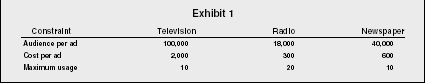
| Constraint | Television | Radio | Newspaper |
| Audience per ad | 100,000 | 18,000 | 40,000 |
| Cost per ad | 2,000 | 300 | 600 |
| Maximum usage | 10 | 20 | 10 |
equations and solves the equations by finding the best solution for the system of equations. This method first finds an initial basic feasible solution and then tries to find a better solution. A series of iterations results in an optimal solution.
SIMPLEX PROBLEM.
Georgia Television buys components that are used to manufacture two television models. One model is called High Quality and the other is called Medium Quality. A weekly production schedule needs to be developed given the following production considerations.
The High Quality model produces a gross profit of $125 per unit, and the Medium Quality model has a $75 gross profit. Only 180 hours of production time are available for the next time period. High Quality models require a total production time of six hours and Medium Quality models require eight hours. In addition, there are only forty-five Medium Quality components on hand.
To complicate matters, only 250 square feet of warehouse space can be used for new production. The High Quality model requires 9 square feet of space while the Medium Quality model requires 7 square feet.
Given the above situation, the simplex method can provide a solution for the production allocation of High Quality models and Medium Quality models.
DYNAMIC PROGRAMMING
Dynamic programming is a process of segmenting a large problem into a several smaller problems. The approach is to solve the all the smaller, easier problems individually in order to reach a solution to the original problem.
This technique is useful for making decisions that consist of several steps, each of which also requires a decision. In addition, it is assumed that the smaller problems are not independent of one another given they contribute to the larger question.
Dynamic programming can be utilized in the areas of capital budgeting, inventory control, resource allocation, production scheduling, and equipment replacement. These applications generally begin with a longer time horizon, such as a year, and then break down the problem into smaller time units such as months or weeks. For example, it may be necessary to determine an optimal production schedule for a twelve-month period.
Dynamic programming would first find a solution for smaller time periods, for example, monthly production schedules. By answering such questions, dynamic programming can identify solutions to a problem that are most efficient or that best serve other business needs given various constraints.
GOAL PROGRAMMING
Goal programming is a technique for solving multi-criteria rather than single-criteria decision problems, usually within the framework of linear programming. For example, in a location decision a bank would use not just one criterion, but several. The bank would consider cost of construction, land cost, and customer attractiveness, among other factors.
Goal programming establishes primary and secondary goals. The primary goal is generally referred to as a priority level 1 goal. Secondary goals are often labeled level 2, priority level 3, and so on. It should be noted that trade-offs are not allowed between higher and lower level goals.
Assume a bank is searching for a site to locate a new branch. The primary goal is to be located in a five-mile proximity to a population of 40,000 consumers. A secondary goal might be to be located at least two miles from a competitor. Given the no trade-off rule, we would first search for a target solution of locating close to 40,000 consumers.
BLENDING PROBLEM.
The XYZ Company mixes three raw materials to produce two products: a fuel additive and a solvent. Each ton of fuel additive is a mixture of 2/5 ton of material A and 3/5 ton of material C. A ton of solvent base is a mixture of 1/2 ton of material A, 1/5 ton of material B, and 3/10 ton of material C. Production is constrained by a limited availability of the three raw materials. For the current production period XYZ has the following quantities of each raw material: 20 tons of material A, 5 tons of material B, and 21 tons of material C. Management would like to achieve the following priority level goals:
Goal 1. Produce at least 30 tons of fuel additive.
Goal 2. Produce at least 15 tons of solvent.
Goal programming would provide directions for production.
INTEGER PROGRAMMING
Integer programming is useful when values of one or more decision variables are limited to integer values. This is particularly useful when modeling production processes for which fractional amounts of products cannot be produced. Integer variables are often limited to two values—zero or one. Such variables are particularly useful in modeling either/or decisions.
Areas of business that use integer linear programming include capital budgeting and physical distribution. For example, faced with limited capital a firm needs to select capital projects in which to invest. This type of problem is represented in Table 1.
As can be seen in the table, capital requirements exceed the available
funds for each year. Consequently, decisions to accept or reject regarding
each of the projects must be made and integer programming would require
the following integer definitions for each of the projects.
x1 = 1 if the new office project is accepted; 0 if rejected
x2 = 1 if the new warehouse project is accepted; 0 if rejected
x3 = 1 if the new branch project is accepted; 0 if rejected
A set of equations is developed from the definitions to provide an optimal solution.
NONLINEAR PROGRAMMING
Nonlinear programming is useful when the objective function or at least one of the constraints is not linear with respect to values of at least one decision variable. For example, the per-unit cost of a product may increase at a decreasing rate as the number of units produced increases because of economies of scale.
STOCHASTIC PROGRAMMING
Stochastic programming is useful when the value of a coefficient in the objective function or one of the constraints is not know with certainty but has a known probability distribution. For instance, the exact demand for a product may not be known, but its probability distribution may be understood. For such a problem, random values from this distribution can be substituted into the problem formulation. The optimal objective function values associated with these formulations provide the basis of the probability distribution of the objective function.
MARKOV PROCESS MODELS
Markov process models are used to predict the future of systems given repeated use. For example, Markov models are used to predict the probability that production machinery will function properly given its past performance in any one period. Markov process models are also used to predict future market share given any specific period's market share.
COMPUTER FACILITY PROBLEM.
The computing center at a state university has been experiencing computer downtime. Assume that the trials of an associated Markov Process are defined as one-hour periods and that the probability of the system being in a running state or a down state is based on the state of the
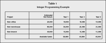
Integer Programming Example
| Project | Estimated Net Return | Year 1 | Year 2 | Year 3 |
| New office | 25,000 | 10,000 | 10,000 | 10,000 |
| New warehouse | 85,000 | 35,000 | 25,000 | 25,000 |
| New branch | 40,000 | 15,000 | 15,000 | 15,000 |
| Available funds | 50,000 | 45,000 | 45,000 |
system in the previous period. Historical data in Table 2 show the transition probabilities.
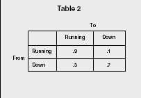
| To | |||
| Running | Down | ||
| From | Running | .9 | .1 |
| Down | .3 | .7 | |
The Markov process would then solve for the following: if the system is running, what is the probability of the system being down in the next hour of operation?
QUEUING THEORY/WAITING
LINE THEORY
Queuing theory is often referred to as waiting line theory. Both terms refer to decision making regarding the management of waiting lines (or queues). This area of management science deals with operating characteristics of waiting lines, such as:
- the probability that there are no units in the system
- the mean number of units in the queue
- the mean number of units in the system (the number of units in the waiting line plus the number of units being served)
- the mean time a unit spends in the waiting line
- the mean time a unit spends in the system (the waiting time plus the service time)
- the probability that an arriving unit has to wait for service
- the probability of n units in the system
Given the above information, programs are developed that balance costs and service delivery levels. Typical applications involve supermarket checkout lines and waiting times in banks, hospitals, and restaurants.
BANK LINE PROBLEM.
XYZ State Bank operates a drive-in-teller window, which allows customers to complete bank transactions without getting out of their cars. On weekday mornings arrivals to the drive-in-teller window occur at random, with a mean arrival rate of twenty-four customers per hour or 0.4 customers per minute.
Delay problems are expected if more than three customers arrive during any five-minute period. Waiting line models can determine the probability that delay problems will occur.
TRANSPORTATION METHOD
The transportation method is a specific application of the simplex method that finds an initial solution and then uses iteration to develop an optimal solution. As the name implies, this method is utilized in transportation problems.
TRANSPORTATION PROBLEM.
A company must plan its distribution of goods to several destinations from several warehouses. The quantity available at each warehouse is limited. The goal is to minimize the cost of shipping the goods. An example of production capacity can be found in Table 3. The forecast for demand is shown in Table 4.
The transportation method will determine the optimal amount to be shipped from each warehouse and determine the optimal destination.
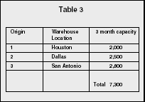
| Origin | Warehouse Location | 3 month capacity |
| 1 | Houston | 2,000 |
| 2 | Dallas | 2,500 |
| 3 | San Antonio | 2,800 |
| Total 7,300 |
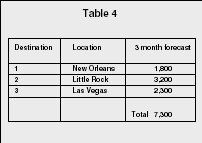
| Destination | Location | 3 month forecast |
| 1 | New Orleans | 1,800 |
| 2 | Little Rock | 3,200 |
| 3 | Las Vegas | 2,300 |
| Total 7,300 |
SIMULATION
Simulation is used to analyze complex systems by modeling complex relationships between variables with known probability distributions. Random values from these probability distributions are substituted into the model and the behavior of the system is observed. Repeated executions of the simulation model provide insight into the behavior of the system that is being modeled.
SEE ALSO: Operations Management ; Operations Scheduling ; Operations Strategy ; Production Planning and Scheduling
Gene Brown
Revised by James J. Cochran
FURTHER READING:
Anderson, David R., Dennis J. Sweeney, and Thomas A. Williams. Quantitative Methods for Business. Cincinnati, OH: South-Western Publishing, 2004.
Blumenfrucht, Israel, and Joel G. Segal. "Updating the Accountant on Financial Advisory Services: Financial Models, Latest Quantitative Techniques, and Other Recent Developments." National Public Accountant, September 1998, 20–23.
Camm, D. Jeffrey, and James R. Evans. Management Science & Decision Technology. Cincinnati, OH: South-Western Publishing, 2000.
McCulloch, C.E., B. Paal, and S.P. Ashdown. "An Optimisation Approach to Apparel Sizing." Journal of the Operational Research Society, May 1998, 492–499.
Comment about this article, ask questions, or add new information about this topic: