BREAK-EVEN POINT
A company's break-even point is the amount of sales or revenues that it must generate in order to equal its expenses. In other words, it is the point at which the company neither makes a profit nor suffers a loss. Calculating the break-even point (through break-even analysis) can provide a simple, yet powerful quantitative tool for managers. In its simplest form, break-even analysis provides insight into whether or not revenue from a product or service has the ability to cover the relevant costs of production of that product or service. Managers can use this information in making a wide range of business decisions, including setting prices, preparing competitive bids, and applying for loans.
BACKGROUND
The break-even point has its origins in the economic concept of the "point of indifference." From an economic perspective, this point indicates the quantity of some good at which the decision maker would be indifferent, i.e., would be satisfied, without reason to celebrate or to opine. At this quantity, the costs and benefits are precisely balanced.
Similarly, the managerial concept of break-even analysis seeks to find the quantity of output that just covers all costs so that no loss is generated. Managers can determine the minimum quantity of sales at which the company would avoid a loss in the production of a given good. If a product cannot cover its own costs, it inherently reduces the profitability of the firm.
MANAGERIAL ANALYSIS
Typically the scenario is developed and graphed in linear terms. Revenue is assumed to be equal for each unit sold, without the complication of quantity discounts. If no units are sold, there is no total revenue ($0). However, total costs are considered from two perspectives. Variable costs are those that increase with the quantity produced; for example, more materials will be required as more units are produced. Fixed costs, however, are those that will be incurred by the company even if no units are produced. In a company that produces a single good or service, this would include all costs necessary to provide the production environment, such as administrative costs, depreciation of equipment, and regulatory fees. In a multi-product company, fixed costs are usually allocations of such costs to a particular product, although some fixed costs (such as a specific supervisor's salary) may be totally attributable to the product.
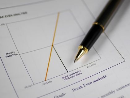
Figure 1 displays the standard break-even analysis framework. Units of output are measured on the horizontal axis, whereas total dollars (both revenues and costs) are the vertical units of measure. Total revenues are nonexistent ($0) if no units are sold. However, the fixed costs provide a floor for total costs; above this floor, variable costs are tracked on a per-unit basis. Without the inclusion of fixed costs, all products for which marginal revenue exceeds marginal costs would appear to be profitable.

Simple Break-Even Analysis: Total Revenues and Total Costs
In Figure 1, the break-even point illustrates the quantity at which total revenues and total costs are equal; it is the point of intersection for these two totals. Above this quantity, total revenues will be greater than total costs, generating a profit for the company. Below this quantity, total costs will exceed total revenues, creating a loss.
To find this break-even quantity, the manager uses the standard profit
equation, where profit is the difference between total revenues and total
costs. Predetermining the profit to be $0, he/she then solves for the
quantity that makes this equation true, as follows:
Let
TR
= Total revenues
TC
= Total costs
P
= Selling price
F
= Fixed costs
V
= Variable costs
Q
= Quantity of output
TR
=
P
×
Q
TC
=
F
+
V
×
Q
TR
−
TC
= profit
Because there is no profit ($0) at the break-even point, TR − TC = 0, and then P × Q − ( F + V × Q ) = 0. Finally, Q = F ( P − V ).
This is typically known as the contribution margin model, as it defines the break-even quantity ( Q ) as the number of times the company must generate the unit contribution margin ( P − V ), or selling price minus variable costs, to cover the fixed costs. It is particularly interesting to note that the higher the fixed costs, the higher the break-even point. Thus, companies with large investments in equipment and/or high administrative-line ratios may require greater sales to break even.
As an example, if fixed costs are $100, price per unit is $10, and variable costs per unit are $6, then the break-even quantity is 25 ($100 ÷ [$10 − $6] = $100 ÷$4). When 25 units are produced and sold, each of these units will not only have covered its own marginal (variable) costs, but will have also have contributed enough in total to have covered all associated fixed costs. Beyond these 25 units, all fixed costs have been paid, and each unit contributes to profits by the excess of price over variable costs, or the contribution margin. If demand is estimated to be at least 25 units, then the company will not experience a loss. Profits will grow with each unit demanded above this 25-unit break-even level.
While it is useful to know the quantity of sales at which a product will
cease to generate losses, it may be even more useful to know the quantity
necessary to generate a desired level of profit, say
D.
TR
−
TC
=
D
P
×
Q
− (
F
+
V
×
Q
) =
D
Then
Q
= (
F
+
D
) ÷ (
P
−
V
)
This has the effect of regarding the desired profit as an increase in the fixed costs to be covered by sales of the product. As the decision-making process often requires profits for payback period, internal rate of return, or net present value analysis, this form may be more useful than the basic break-even model.
BASIC ASSUMPTIONS
There are several assumptions that affect the applicability of break-even analysis. If these assumptions are violated, the analysis may lead to erroneous conclusions.
It is tempting to the manager to set the contribution margin (and thus the price) by using the sales goal (or certain demand) as the quantity. However, sales goals and market demand are not necessarily equivalent, especially if the customer is price-sensitive. Price-elasticity exists when customers will respond positively to lower prices and negatively to higher prices, and is particularly applicable to nonessential products. A small change in price may affect the sale of skis more than the sale of insulin, an inelastic-demand item due to its inherently essential nature. Therefore, using this method to set a prospective price for a product may be more appropriate for products with inelastic demand. For products with elastic demand, it is wiser to estimate demand based on an established, acceptable market price.
Typically, total revenues and total costs are modeled as linear values, implying that each unit of output incurs the same per-unit revenue and per-unit variable costs. Volume sales or bulk purchasing may incorporate quantity discounts, but the linear model appears to ignore these options.
A primary key to detecting the applicability of linearity is determining the relevant range of output. If the forecast of demand suggests that 100 units will be demanded, but quantity discounts on materials are applicable for purchases over 500 units from a single supplier, then linearity is appropriate in the anticipated range of demand (100 units plus or minus some fore-cast error). If, instead, quantity discounts begin at 50 units of materials, then the average cost of materials may be used in the model. A more difficult issue is that of volume sales, when such sales are frequently dependent on the ordering patterns of numerous customers. In this case, historical records of the proportionate quantity-discount sales may be useful in determining average revenues.
Linearity may not be appropriate due to quantity sales/purchases, as noted, or to the step-function nature of fixed costs. For example, if demand surpasses the capacity of a one-shift production line, then a second shift may be added. The second-shift supervisor's salary is a fixed-cost addition, but only at a sufficient level of output. Modeling the added complexity of nonlinear or step-function costs requires more sophistication, but may be avoided if the manager is willing to accept average costs to use the simpler linear model.
One obviously important measure in the break-even model is that of fixed costs. In the traditional cost-accounting world, fixed costs may be determined by full costing or by variable costing. Full costing assigns a portion of fixed production overhead charges to each unit of production, treating these as a variable cost. Variable costing, by contrast, treats these fixed production overhead charges as period charges; a portion of these costs may be included in the fixed costs allocated to the product. Thus, full costing reduces the denominator in the break-even model, whereas the variable costing alternative increases the denominator. While both of these methods increase the break-even point, they may not lend themselves to the same conclusion.
Recognizing the appropriate time horizon may also affect the usefulness of break-even analysis, as prices and costs tend to change over time. For a prospective outlook incorporating generalized inflation, the linear model may perform adequately. Using the earlier example, if all prices and costs double, then the break-even point Q = 200 ÷ (20 − 12) = 200 ÷ 8 = 25 units, as determined with current costs. However, weakened market demand for the product may occur, even as materials costs are rising. In this case, the price may shift downward to $18 to bolster price-elastic demand, while materials costs may rise to $14. In this case, the break-even quantity is 50 (200 ÷ [18 − 14]), rather than 25. Managers should project break-even quantities based on reasonably predictable prices and costs.
It may defy traditional thinking to determine which costs are variable and which are fixed. Typically, variable costs have been defined primarily as "labor and materials." However, labor may be effectively salaried by contract or by managerial policy that supports a full workweek for employees. In this case, labor should be included in the fixed costs in the model.
Complicating the analysis further is the concept that all costs are variable in the long run, so that fixed costs and the time horizon are interdependent. Using a make-or-buy analysis, managers may decide to change from in-house production of a product to subcontracting its production; in this case, fixed costs are minimal and almost 100 percent of the costs are variable. Alternatively, they may choose to purchase cutting-edge technology, in which case much of the variable labor cost is eliminated; the bulk of the costs then involve the (fixed) depreciation of the new equipment. Managers should project break-even quantities based on the choice of capital-labor mix to be used in the relevant time horizon.
Traditionally, fixed costs have been allocated to products based on estimates of production for the fiscal year and on direct labor hours required for production. Technological advances have significantly reduced the proportion of direct labor costs and have increased the indirect costs through computerization and the requisite skilled, salaried staff to support company-wide computer systems. Activity-based costing (ABC) is an allocation system in which managers attempt to identify "cost drivers" which accurately reflect the appropriate usage of fixed costs attributable to production of specific products in a multi-product firm. This ABC system tends to allocate, for example, the CEO's salary to a product based on his/her specific time and attention required by this product, rather than on its proportion of direct labor hours to total direct labor hours.
EXTENSIONS OF BREAK-EVEN ANALYSIS
Break-even analysis typically compares revenues to costs. However, other models employ similar analysis.
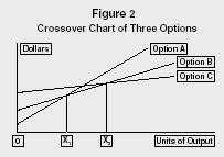
Crossover Chart of Three Options
In the crossover chart, the analyst graphs total-cost lines from two or more options. These choices may include alternative equipment choices or location choices. The only data needed are fixed and variable costs of each option. In Figure 2, the total costs (variable and fixed costs) for three options are graphed. Option A has the low-cost advantage when output ranges between zero and X units, whereas Option B is the least-cost alternative between X and X units of output. Above X units, Option C will cost less than either A or B. This analysis forces the manager to focus on the relevant range of demand for the product, while allowing for sensitivity analysis. If current demand is slightly less than X Option B would appear to be the best choice. However, if medium-term forecasts indicate that demand will continue to grow, Option C might be the least-cost choice for equipment expected to last several years. To determine the quantity at which Option B wrests the advantage from Option A, the manager sets the total cost of A equal to the total cost of B ( F A + V A × Q = F B + V B × Q ) and solves for the sole quantity of output ( Q ) that will make this equation true. Finding the break-even point between Options B and C follows similar logic.
The Economic Order Quantity (EOQ) model attempts to determine the least-total-cost quantity in the purchase of goods or materials. In this model, the total of ordering and holding costs is minimized at the quantity where the total ordering cost and total holding cost are equal, i.e., the break-even point between these two costs.
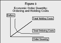
Economic Order Quantity: Ordering and Holding Costs
As companies merge, layoffs are common. The newly formed company typically enjoys a stock-price surge, anticipating the leaner and meaner operations of the firm. Obviously, investors are aware that the layoffs reduce the duplication of fixed-cost personnel, leading to a smaller break-even point and thus profits that begin at a lower level of output.
APPLICATIONS IN SERVICE INDUSTRIES
While many of the examples used have assumed that the producer was a manufacturer (i.e., labor and materials), break-even analysis may be even more important for service industries. The reason for this lies in the basic difference in goods and services: services cannot be placed in inventory for later sale. What is a variable cost in manufacturing may necessarily be a fixed cost in services. For example, in the restaurant industry, unknown demand requires that cooks and table-service personnel be on duty, even when customers are few. In retail sales, clerical and cash register workers must be scheduled. If a barber shop is open, at least one barber must be present. Emergency rooms require round-the-clock staffing. The absence of sufficient service personnel frustrates the customer, who may balk at this visit to the service firm and may find competitors that fulfill the customer's needs.
The wages for this basic level of personnel must be counted as fixed costs, as they are necessary for the potential production of services, despite the actual demand. However, the wages for on-call workers might be better classified as variable costs, as these wages will vary with units of production. Services, therefore, may be burdened with an extremely large ratio of fixed-to-variable costs.
Service industries, without the luxury of inventoriable products, have developed a number of ways to provide flexibility in fixed costs. Professionals require appointments, and restaurants take reservations; when the customer flow pattern can be predetermined, excess personnel can be scheduled only when needed, reducing fixed costs. Airlines may shift low-demand flight legs to smaller aircraft, using less fuel and fewer attendants. Hotel and telecommunication managers advertise lower rates on weekends to smooth demand through slow business periods and avoid times when the high-fixed-cost equipment is underutilized. Retailers and banks track customer flow patterns by day and by hour to enhance their short-term scheduling efficiencies. Whatever method is used, the goal of these service industries is the same as that in manufacturing: reduce fixed costs to lower the break-even point.
Break-even analysis is a simple tool that defines the minimum quantity of sales that will cover both variable and fixed costs. Such analysis gives managers a quantity to compare to the forecast of demand. If the break-even point lies above anticipated demand, implying a loss on the product, the manager can use this information to make a variety of decisions. The product may be discontinued or, by contrast, may receive additional advertising and/or be re-priced to enhance demand. One of the most effective uses of break-even analysis lies in the recognition of the relevant fixed and variable costs. The more flexible the equipment and personnel, the lower the fixed costs, and the lower the break-even point.
It is difficult to overstate the importance of break-even analysis to sound business management and decision making. Ian Benoliel, CEO of management software developer NumberCruncher.com, said on Entrepreneur.com (2002):
The break-even point may seem like Business 101, yet it remains an enigma to many companies. Any company that ignores the break-even point runs the risk of an early death and at the very least will encounter a lot of unnecessary headaches later on.
SEE ALSO: Activity-Based Costing ; Cost Accounting ; Cost-Volume-Profit Analysis ; Financial Issues for Managers
Karen L. Brown
Revised by Laurie Hillstrom
FURTHER READING:
Benoliel, Ian. "Calculating Your Breakeven Point." Entrepreneur.com (25 March 2002). < http://www.entrepreneur.com/article/0,4621,298145,00.html >.
"Breakeven Analysis." Business Owner's Toolkit. Available from < http://www.toolkit.cch.com/text/P06_7530.asp >.
Deal, Jack. "The Break-Even Point and the Break-Even Margin." BusinessKnow-How.com. Available from < http://www.businessknowhow.com/money/breakeven.htm >.
Garrison, Ray H., and Eric W. Noreen. Managerial Accounting. Boston: Irwin/McGraw-Hill, 1999.
Horngren, Charles T., George Foster, and Srikant M. Datar. Cost Accounting: A Managerial Emphasis. Upper Saddle River, NJ: Prentice Hall, 1997.
Render, Barry, and Jay Heizer. Principles of Operations Management. Upper Saddle River, NJ: Prentice Hall, 1997.
Person is 55 can take retirement for 625.63 monthly but if she waits when she is 62 would make 977.55 monthly. When would her breakeven point be?